What About Prices?

Chapter 8 from my forthcoming book Rebuilding Economics from the Top Down

Inflation, having been quiescent for decades, became a serious issue once more with the bout of inflation that occurred after the peak of the government reaction to the Covid crisis. Though it did not reach the 12-15% levels of the mid-1970s to mid-1980s, and it has fallen sharply from its peak of 8.9% p.a. in June of 2022 to 3.2% in October 2023, it was still a serious break from the low inflation period from the mid-1980s until the beginning of the 2020s—see the top chart in Figure 19.

This is Chapter 8 from my forthcoming book Rebuilding Economics from the Top Down, which will be published by the Budapest Centre for Long-Term Sustainability and the Pallas Athéné Domus Meriti Foundation. I am serialising the book chapters here. A watermarked PDF of the manuscript is available to supporters.

The original Neoclassical (and Austrian) explanation for inflation is that it is caused by "too much money chasing too few goods", with government money creation being the culprit, and with "long and variable lags" between government deficits and actual inflation:

The lag between the creation of a government deficit and its effects on the behavior of consumers and producers could conceivably be so long and variable that the stimulating effects of the deficit were often operative only after other factors had already brought about a recovery rather than when the initial decline was in progress. Despite intuitive feelings to the contrary, I do not believe we know enough to rule out completely this possibility. If it were realized, the proposed framework could intensify rather than mitigate cyclical fluctuations; that is, long and variable lags could convert the fluctuations in the government contribution to the income stream into the equivalent of an additional random disturbance. (Friedman 1948, p. 254. Emphasis added)

This explanation appeared to get some support from the unprecedented peacetime deficits run because of Covid. It also justified the conventional Federal Reserve policy response to inflation, of increasing the interest rate. However, the non-mainstream economist Isabella Weber argued in The Guardian that price controls, and not interest rates, should be used to control this rate of inflation, and that its main cause was not excessive aggregate demand, but supply bottlenecks caused by Covid, followed by excessive profit margins.

Her argument, which caused a predictable outrage amongst and ridicule from mainstream economists, was backed by her empirical research (Weber and Wasner 2023; Weber et al. 2022; Weber 2022), which was based on a tradition of non-mainstream analysis of price-setting that emanated from the great Polish economist Michal Kalecki (Kalecki 1971; Kalecki 1954, 1949, 1942b, 1941, 1938). Isabella enjoyed the last laugh in this debate, as her explanation of inflation was vindicated, and she became one of the few non-mainstream economists to achieve widespread mainstream media recognition.

In this chapter, I will use Kalecki's pricing equation to extend the dynamic non-equilibrium monetary model developed in the previous chapter, to show the flexibility and realism inherent in developing macroeconomics from macroeconomic definitions.

Figure 19: USA Post WWII Inflation, Government Surplus, Federal Funds Rate and Nonfinancial Sector Profits

A Kaleckian Pricing Equation

To define the aggregate price level P, we need to distinguish between nominal and "real" output. Using Y_N for nominal output and Y_R for real output, we have:

I express it this way because, though economics habitually work in terms of "real" GDP, this is in fact a term which is derived from the actual, recorded nominal GDP, and an aggregate price level that is also derived from nominal GDP data.

We can replace real output with employment L times the output to labour ratio Y_L^r, once we update equation to use Y_R instead of Y:

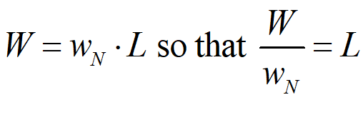
Next, we can replace L with the money wage bill W divided by the nominal wage w_N:

Finally, we can replace W with the wages share of GDP times nominal output:

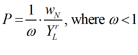
Now we can express the price level as a function of the wages share of GDP, nominal output, and the output to labour ratio. Equation combines all the substitutions above:

This reduces to:

This is true as an algebraically derived expression which applies in equilibrium, but it excludes the pricing decisions of firms as a causal factor in price setting. As the microeconomic research in Chapter 5 showed, real-world firms are price-setters. They do not respond mechanically to a "downward-sloping market demand curve", but rather each firm sets a price at which it will sell its differentiated product. That price is well above its average variable costs at all output levels, and above the sum of average variable and fixed costs at its target output level. The firm then tries to sell as many units as possible, predominantly at the expense of its rival's sales. Since real-world firms experience either constant or very slowly falling marginal costs, the ratio of Price to Variable costs is relatively insensitive to the quantity of output (though the markup over total costs V+F/q increases as output rises, given falling per unit fixed costs). Using the Greek letter  (the equivalent of the English letter m) for this microeconomic ratio, we have:

Here , while it is effectively constant with respect to a firm's output, is a decision variable for individual firms. It is an outcome of both the competitive forces which firms exert on each other, and the state of aggregate demand, which determines overall demand for a given market.

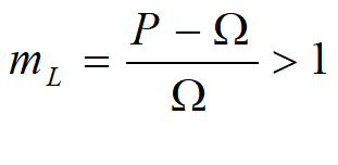
Labour is only one of many variable costs—the other key components being energy, and raw material inputs to production—but Labour is already part of the price formula derived in Equation , whereas they are not. Defining  as the per unit wage cost, we therefore define the aggregate markup of prices over wage cost, for which I use the symbol m_L:

Replacing  with m_L in Equation gives us an expression in which firms do have agency, in the form of an average markup on the labour costs of production:

This is equivalent to Kalecki's markup pricing equation, where Kalecki explained the size of the markup by what he called the "degree of monopoly" (Kalecki 1954, p. 13). The false Marshallian rising-marginal-cost tinges of this expression can be dispensed with by instead calling it the "degree of competition". Using the ^ notation, we can now define the inflation rate:

We can use this formula to decompose the causes of inflation into change in the average markup, change in the median wage, and change in "labor productivity". This decomposition confirms Weber's analysis that change in the average markup, and not change in the median wage, was the main contributor to the Covid inflation—see Figure 20:

Figure 20: Decomposition of contributions to Us Inflation 2018-2023, with the budget deficit on the right-hand Y axis

Table 7 shows that both before and during Covid, changes in the markup normally exceeded the rate of inflation, while wage changes normally fell below it—except for the three quarters before the Covid emergency began, and the first four quarters of that emergency.

Table 7: US 2018-2023 data highlighting when markup and wage changes exceeded the rate of inflation

In fact, over the whole period from 1980 till 2023, the average change on the markup (5.1% p.a.) exceeded average inflation itself (3.3%), while the average change in the money wage (1.8%) was below the inflation rate—with the increased output to labour ratio (3.6%), which proxies technological change, deducting from inflation to make up the difference.

This analysis also shows that the markup is, as Kalecki observed, a variable rather than a constant:

The simplest interpretation … is to admit that gross profit margins P-C tend to fall and rise with the unit prime costs C. Of course, they need not change in exactly the same proportion, because "my" degree of monopoly cannot be assumed to remain constant. (Kalecki 1942a, p. 127)

However, while much ink has been spilt on the issue of how change in money wages is determined, very little has been devoted to the topic of what determines markups. Kalecki is also effectively arguing that Price minus Variable Cost is approximately a constant times Variable Cost. Though this is obviously an incomplete causal argument, it justifies treating the m_L as a constant as a first approximation in modelling, and as determined by a desired markup level as a second approximation.

These models show that, contrary to the biases of Neoclassical and Austrian economists, prices—at least in the form of an aggregate price level—can be a destabilizing rather than a stabilizing factor in macroeconomics in the presence of private debt.

A Monetary Model with Prices

With prices introduced—at this stage in the form only of a generalised price level—we have a difference between real and nominal output:

This has the obvious verbal rendition that "change in the percentage rate of growth of nominal output is the sum of change in real output and change in the price level". We now integrate this with the pure credit economy model developed in the previous section. Our basic definitions are:

With price dynamics modelled as a first-order time lag convergence to the equilibrium given by equation , the dynamic rendition of these definitions is:

The rate of growth of the employment ratio equation is unchanged, but all the other equations now include price dynamics, in addition to the "real" dynamics outlined in the previous section, given the presence of nominal output Y_N in each of the equations.

As shown in the Appendix, this generates the following set of differential equations:

When this system is simulated without debt, the dynamics shown in Figure 21 result. Price dynamics cause the system to stabilize, as mainstream economists expect.

Figure 21: Prices stabilize a system without private debt

However, when private debt is included, the dynamics shown in Figure 22 result. Rather than prices stabilizing the system, the rate of change of prices turns negative, so that deflation causes the private debt to GDP ratio to rise over time. This leads to the debt ratio exploding and, ultimately, the rate of economic growth collapsing.

Figure 22: Price dynamics lead to a debt deflation with private debt

This phenomenon was first identified by Irving Fisher in his paper "The Debt-Deflation Theory of Great Depressions". What I term "Fisher's Paradox" is that "The more the debtors pay, the more they owe":

deflation caused by the debt reacts on the debt. Each dollar of debt still unpaid becomes a bigger dollar, and if the over-indebtedness with which we started was great enough, the liquidation of debts cannot keep up with the fall of prices which it causes.

In that case, the liquidation defeats itself. While it diminishes the number of dollars owed, it may not do so as fast as it increases the value of each dollar owed. Then, the very effort of individuals to lessen their burden of debts increases it, because of the mass effect of the stampede to liquidate in swelling each dollar owed.

Then we have the great paradox which, I submit, is the chief secret of most, if not all, great depressions: The more the debtors pay, the more they owe. The more the economic boat tips, the more it tends to tip. It is not tending to right itself, but is capsizing. (Fisher 1933, p. 344. Italic emphasis added)

This phenomenon is brutally evident in the US data for 1920-1940—see Figure 23.

Figure 23: Debt, Deflation and Depression in the USA 1920-1940

The rising nominal GDP, private debt and price levels of the 1920s gave way to falling GDP, debt and prices in the 1930s, but the rate of decrease of GDP was so much greater than the rate of decrease of private debt that the debt ratio actually rose until 1932. Then the recovery of GDP largely engineered by the New Deal stopped the collapse of prices and both real and nominal GDP, leading to a falling private debt ratio and the end of the worst of the Great Depression.

Therefore, "The more the debtors pay, the more they owe" is not merely a clever phrase, but an accurate description of what happened during the Great Depression. The price mechanism, of which mainstream economists are so enamoured, is a potential source on instability, rather than stability, in a capitalist economic system with finance. There is no more fitting way to end this chapter than to quote Hyman Minsky, the great successor to Irving Fisher, on the need to abandon the Neoclassical paradigm and its obsession with equilibrium:

Instability is an observed characteristic of our economy. For a theory to be useful as a guide to policy for the control of instability, the theory must show how instability is generated. The abstract model of the neoclassical synthesis cannot generate instability. When the neoclassical synthesis is constructed, capital assets, financing arrangements that center around banks and money creation, constraints imposed by liabilities, and the problems associated with knowledge about uncertain futures are all assumed away. For economists and policymakers to do better we have to abandon the neoclassical synthesis. (Minsky 1982, p. xiii)

Appendix: Deriving the Price-Based Model

Price dynamics are included in the wages share equation as follows:

Then the private debt ratio:

The system of equations is now: