The Role of the Price Level

This is chapter 8 of my forthcoming book Money and Macroeconomics from First Principles, for Elon Musk and Other Engineers

The price level is introduced into these models via a version of Kalecki’s markup pricing equation {Kalecki, 1954 #7115`, p. 16}. The essence of Kalecki’s formula is that prices are set as a markup on the prime cost of production, which can be reduced (in a simple scalar model) to the nominal wage divided by the output to labour ratio.[1] As with the differential equations of the previous chapter, this can be derived from first principles.

Define the price level P as the ratio of nominal output Y_N to real output Y_R. The nominal wage (w_N) takes the place of the real wage w used in the previous chapter. We then decompose the price level into the inverse of the wages share of GDP times the nominal wage divided by the output to labor ratio.

This is an algebraic manipulation that gives no agency to firms. We introduce agency by substituting the inverse of the wages share of GDP with the markup on labour costs m_L:

Modeling inflation as a time-lagged convergence to the equilibrium level of prices given by Equation yields Equation :

It is easy to show that price dynamics impact the rate of growth of workers share of output, the private debt to GDP ratio, and the net government spending to GDP ratio:

The effect of price dynamics vary depending across the three models developed in the previous chapter. In the 2D model with wage share and employment dynamics, the price level functions as an equilibrating force. Whereas the model without price dynamics generates sustained cycles, the model with price dynamics converges to equilibrium—see Figure 29.

Figure 29: Price dynamics stabilize the 2-dimensional model

However, when the private debt ratio is included, a very different phenomenon emerges: a “debt-deflation”. As noted in Chapter 5, this was Irving Fisher’s explanation for why the Great Depression was so severe: a falling price level amplifies the private debt to GDP ratio, leading to a growth in the debt to GDP ratio even if borrowing has ceased, or even turned negative—see Figure 30.

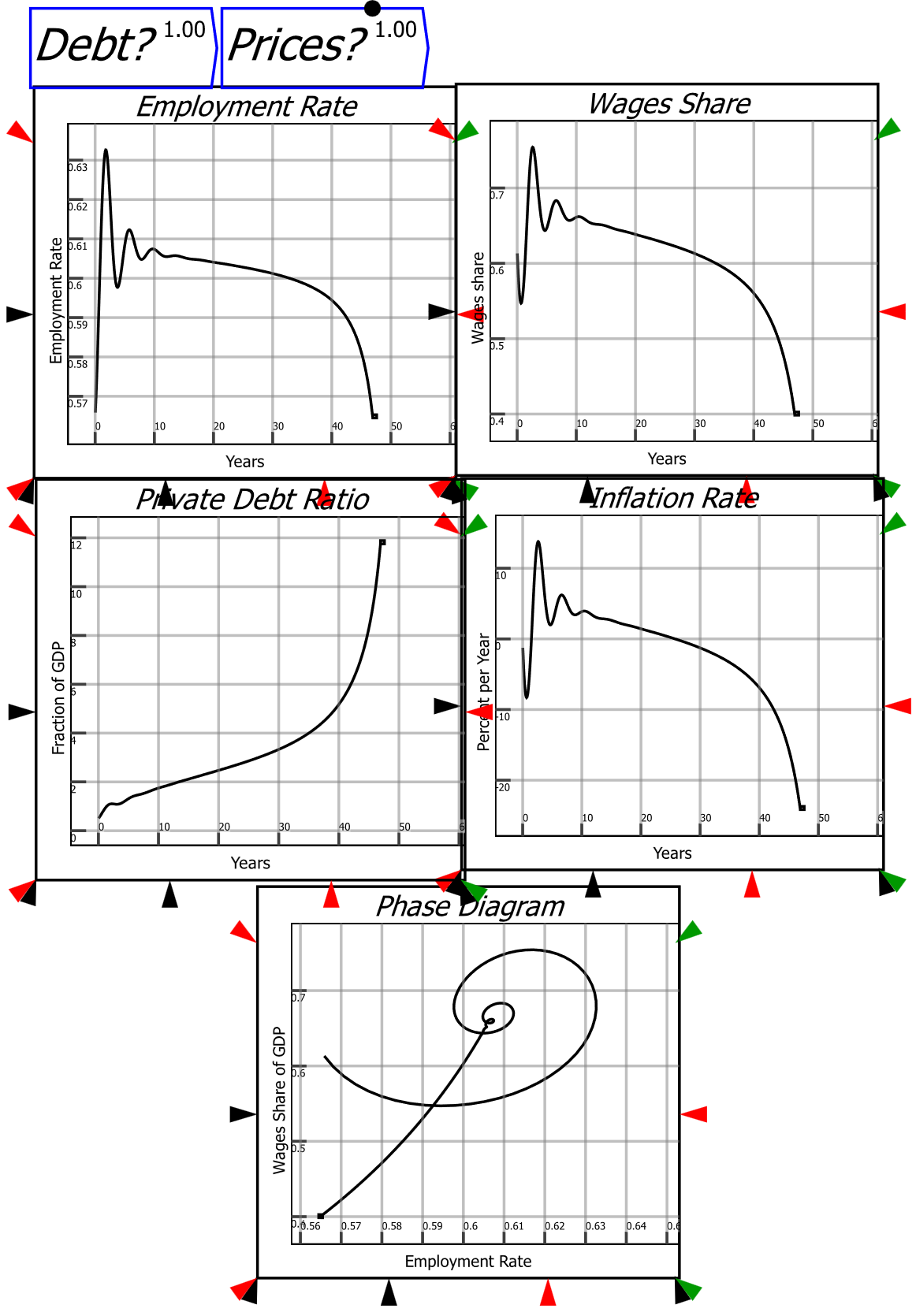
Figure 30: A debt-deflationary collapse

With government spending, this calamitous outcome is avoided—see Figure 31.

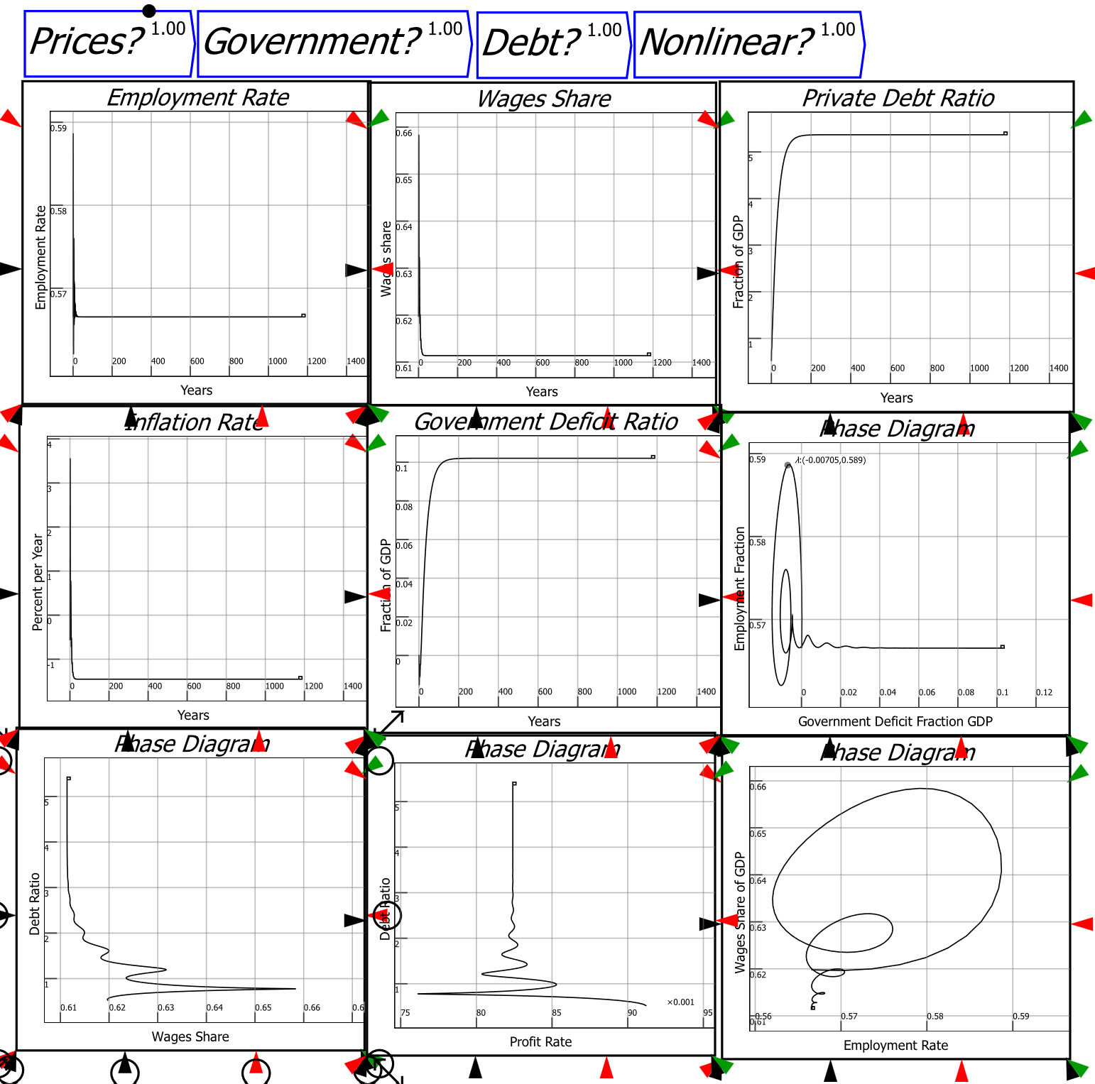
Figure 31: A government deficit prevents a debt-deflationary collapse

The government’s counter-cyclical spending prevents a crisis, as Minsky argued:

With the rise of big government, the reaction of tax receipts and transfer payments to income changes implies that any decline in income will lead to an explosion of the government deficit. Since it can be shown that profits are equal to investment plus the government’s deficit, profit flows are sustained whenever a fall in investment leads to a rise in the government’s deficit. A cumulative debt deflation process that depends on a fall of profits for its realization is quickly halted when government is so big that the deficit explodes when income falls. {Minsky, 1982 #35`, p. xxviii }

This highlights the issue noted in the previous chapter, that running a balanced budget removes a stabilizing factor from the system, thus exposing the economy to the possibility of another debt-deflation.

An Expected Riposte

One obvious riposte to the argument that government spending stabilizes an unstable economy is that money creation simply creates inflation. Therefore, government spending that is not taxed away is instead eroded by inflation. Musk has made both these assertions in recent times:

“If we address the massive waste in the government, then we can actually address the inflation. So provided the economy grows faster than the money supply, which means you stop the government overspending, you have no inflation.” https://x.com/MrPitbull07/status/1895513318338826356 (28 Feb 2025)

“Inflation, throughout history, has been used as a pernicious tax. It's like one degree removed, so people don't feel it directly. Then, the politicians will try to blame it on something else. But it's all about government spending.” https://x.com/ElonClipsX/status/1862356258369479098 (29 Nov 2024)

There are logical and empirical flaws with this riposte.

Firstly, even if it were true that, as Milton Friedman once asserted, the “Inflation is always and everywhere a monetary phenomenon in the sense that it is and can be produced only by a more rapid increase in the quantity of money than in output”,[2] new money is created not only by the government, but also by private banks. The government deficit alone is not the only cause of new money creation, and in practice, the deficit is normally much smaller than credit (see Figure 17 on page 26).

Secondly, the causality between money supply growth and inflation is arguably the reverse of this assumed process: inflation may cause money supply growth, rather than vice versa. This is especially true of credit money, as Basil Moore pointed out in “Unpacking the post Keynesian black box: bank lending and the money supply” {Moore, 1983 #126}. Lines of credit for corporations, and unused credit card limits for consumers, means that if an increase is spending is necessitated by a rise in prices, then the money supply expands in concert:

Changes in bank lending have been the proximate source of annual changes in the money stock over the past fifteen years. The credit crunch of 1966 spurred a widespread move toward formalizing, in a legally obligating manner, the hitherto largely informal credit-line arrangements prevailing between banks and their business customers. Corporations wanted and were willing to pay for legally-binding credit lines. The controllability of bank lending to business corporations appears distinctly limited. {Moore, 1983 #126`, p. 544}

As a result, the money supply is not a constraint to inflation, but accommodative of inflation.

The degree to which the money supply is accommodative is highlighted by Figure 32, which shows that unused credit provisions rose from 10% of the Broad Money supply in 1990 to 60% when the GFC began. Though they fell sharply then, and again when Broad Money was dramatically expanded by government schemes during Covid, unused credit still exceeds 20% of the Broad Money supply. There is therefore plenty of room for inflation—in consumer prices, energy costs, wage costs, and supply chain disruptions—to cause an increase in credit use, and therefore an increase in the money supply.

Figure 32: Unused credit lines compared to Broad Money

The main causes of inflation are then those indicated by Kalecki’s markup-pricing equation, Equation . These are increases in firm markups, increases in money wages, and changes in the output to labour ratio (AKA “labour productivity”).

Fundamentally, rather than changes in the money supply causing inflation, struggles over the distribution of income, and changes in the conditions of production, cause inflation—see Figure 33.

Figure 33: Decomposing inflation into change in markups, money wages, and labour productivity

These changes in prices then cause changes in the money supply. The iron link between the government deficit and the rate of inflation, hypothesised by Friedman, and accepted by many economic commentators today, does not exist. This is one reason for the inverse correlation between inflation and government money creation, versus the positive but still minor correlations between credit and inflation—see Figure 34.

Figure 34: Correlations between changes in money sources and inflation

There is one field in which a causal link between one form of money creation and inflation is very strong, however: the prices of nonfinancial asset like house and shares.

Nonfinancial Assets

The monetary arguments in the preceding chapters have considered financial assets, which are claims on other entities in a financial system. Since there is a matching liability for every asset, the sum of all financial assets and liabilities is zero. This constitutes a conservation law, whose consequences must be understood to properly consider assertions about monetary dynamics. Many widely-believed monetary propositions contradict this conservation law, and are therefore false.

In contrast, a nonfinancial asset is an asset for which there is no offsetting liability. These include houses and factories, which are assets to their owners but liabilities to no-one—even if a financial asset like a mortgage is attached to them. It also includes shares in excess of their limited liability valuation. These are not monetary entities, but their value is expressed in monetary terms as the price they are expected to yield if sold at current market prices. The sum of nonfinancial assets is clearly positive.

However, the summation itself is hypothetical only, since if all owners of a particular class of nonfinancial assets—say, residential houses—tried to liquidate their assets at once, the market price would collapse. The realization of the estimated financial value of a nonfinancial asset thus relies upon only a small and relatively stable fraction of such assets being sold at any point in time.

Nonfinancial assets are often purchased primarily using credit—that is, by a change in the level of private debt.

Inflating—and Rescuing—Asset Prices

The previous chapter showed that credit is a key component of aggregate demand and income. The fact that credit is also used to buy nonfinancial assets means that it is not possible to neatly separate macroeconomics from finance. Credit plays a critical role in asset markets: mortgage debt in the housing market, and margin debt in the share market.

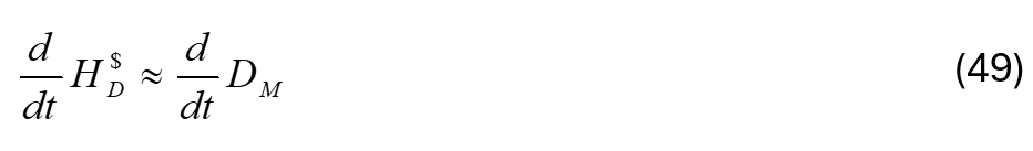
Since mortgages in advanced economies account for of the order of 70% and above of the purchase price of a house, at a first pass, one can assume that the monetary demand for housing is equal to the change in the level of mortgage debt. Using H_D^$ for aggregate housing demand in money terms, and D_M for mortgage debt, this yields:

Using H_D for demand for physical houses per year, and H_P for the price of a “representative” house, then the demand for housing in terms of houses per year is:

The annual supply of housing H_S consists of the time-varying fraction h of the existing housing stock Q_H that is put up for sale, plus the net creation of new houses per year:

Since the housing stock varies much more slowly than debt, for simplicity we can drop the rate of change of the housing stock term and consider simply the proportion h of existing houses offered for sale. If price adjusted instantaneously to match the physical flows of supply and demand, then I could write:

So that P_H would be given by:

Treating the rates of change of h and H_Q as negligible, this implies that the rate of change of house prices is related to—and largely driven by—the acceleration of mortgage debt:

This relationship is confirmed by the data—see Figure 35 (where the differentials have been normalized by dividing by the House Price Index and GDP respectively).[3] Though the correlations of both Household Debt[4] to the House Price Index and household credit to change in the House Price Index are both positive, the largest correlation unaffected by collinearity is between the second difference of household debt and the first difference of house prices, as implied by Equation —see Figure 35. [5]

Figure 35: The relationship between household debt and house prices

Mainstream finance theory, in the form of the “Modigliani-Miller Hypothesis” , asserts that leverage has no impact on share market valuations:

We conclude therefore that levered companies cannot command a premium over unlevered companies because investors have the opportunity of putting the equivalent leverage into their portfolio directly by borrowing on personal account. {Modigliani, 1958 #4632`, p. 273}

This is strongly contradicted by the data, which shows a staggering correlation between change in margin debt and the Cyclically Adjusted Price to Earnings (CAPE) ratio over the last century—see Figure 36.[6]

Figure 36: A century of margin debt and share market valuations

The coincidence of booms and busts in asset prices with macroeconomic booms and busts is thus no coincidence: the huge asset overvaluations of 1929, 2000, 2007 and the mid-2020s are driven by the same factors which caused the booms and busts of the macroeconomy itself. Asset price bubbles are driven by credit bubbles, which burst if for no other reason than their persistence depends on ever-accelerating levels of private debt.

These asset price bubbles are damaging aspects of private money creation. While the debt-deflationary forces modelled in the previous chapters on their own explain economic collapses caused by excessive private debt, the fact that margin debt reached 8.9% of GDP in 1929, when margin loans allowed up to a factor leverage, shows why the Great Crash of 1929 was so devastating. This use of private credit is far more destructive than it is creative.

A Realistic Pricing Equation

Mainstream (Neoclassical) economists would reject the Kaleckian pricing equation used here, on the grounds that prices are set by supply and demand, and not merely by a markup on wage costs per unit of output. The basis of the Neoclassical model of price determination is that firms maximise their profits by equating marginal revenue to marginal cost, where marginal revenue declines with output, and marginal cost rises.

This model is based on a series of abstractions from the real world. Firms are assumed to sell homogeneous products, which means that price is the only means by which firms compete. Consumers are assumed to have complete information, so that all firms sell at the market price: any firm who prices above that level gets no sales, while any firm pricing below it will be overwhelmed with customers.

However, real-world competition is characterized by heterogeneity: there is a car market, but there is no such thing as a homogeneous car, let alone an equilibrium price for it. Consumers have incomplete information.

Similarly, numerous surveys of how firms set prices have found that the typical firm has constant or falling marginal cost—not the rising marginal cost assumed by economists. The last person to discover this was the then Vice-Chair of the Federal Reserve, and Vice-President of the American Economic Association. He reported that:

Another very common assumption of economic theory is that marginal cost is rising. This notion is enshrined in every textbook and employed in most economic models. It is the foundation of the upward-sloping supply curve…

The overwhelmingly bad news here (for economic theory) is that, apparently, only 11 percent of GDP is produced under conditions of rising marginal cost.33F[7] {Blinder, 1998 #297`, pp. 101-102. Emphasis added}

This is because, in the real world, factories are designed by engineers to reach peak performance at or very near capacity. As Eiteman put it in 1947, engineers design factories:

so as to cause the variable factor to be used most efficiently when the plant is operated close to capacity. Under such conditions an average variable cost curve declines steadily until the point of capacity output is reached. A marginal curve derived from such an average cost curve lies below the average curve at all scales of operation short of peak production, a fact that makes it physically impossible for an enterprise to determine a scale of operations by equating marginal cost and marginal revenues unless demand is extremely inelastic. {Eiteman, 1947 #1192`, p. 913}

This analysis has been confirmed by about 70 surveys {Lee, 1998 #1090}, all of which have found that the actual cost structure of firms is as shown in Figure 37, taken from {Andrews, 1949 #6865}: average fixed costs are a rectangular hyperbola, while variable costs per unit are either constant or falling as production volume increases out to plant capacity.

Figure 37: Andrews' sketch of the cost structure of the typical firm {Andrews, 1949 #6865`, p. 80}

This implies an alternative model of competition and pricing. Firms produce differentiated products, and sell them at a list price P, which is set, as in Kalecki’s pricing equation, by a markup on average variable costs V. Fixed cost per unit of output falls as a rectangular hyperbola as output increases. This empirically-based vision of firm costs and revenues is shown in Figure 38

Figure 38: Profit, Revenue and Costs at the target output level for the representative firm

The profits of the firm P are given by Equation :

The differential of profit with respect to the quantity sold is therefore always positive:

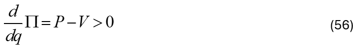
Therefore, as Eiteman said, the best strategy for the firm is to sell as many units as it can. Since its competitors are all trying to do the same thing, while market demand is, for mature industries, a relatively stable fraction of GDP, this leads to the evolutionary competitive struggle we witness in most real-world markets. Firms compete by product differentiation, with the successful innovators coming to dominate the industry, but they remain subject to evolutionary competition from all other firms in the industry. Given this dynamic, then rather than industries being characterized by the standard Neoclassical taxonomy, with monopoly at one extreme and perfect competition at the other, industries are characterized by a power law distribution of firm sizes {Axtell, 2001 #6302}.

We can build a more informative analysis of actual profit maximizing behaviour by considering, not total profit, but profit per unit:

The differential of profit per unit with respect to q is:

This is obviously identical to the negative of the differential of fixed cost per unit:

In words, Equation says that the increase in profit per unit is identical to the fall in fixed cost per unit. This is the essence of the real-world profit maximization strategy: to reduce fixed cost per unit by increasing sales. Profit per unit then rises precisely as much as fixed cost per unit falls. This changes the focus of attention from the Neoclassical obsession with marginal costs—which manufacturers have revealed in numerous surveys is of little importance to actual production decisions, since it is normally either constant or falling and well below price (and “marginal revenue”)—to average fixed costs, and both setting a price and achieving a sales target which substantially exceeds the breakeven point (where total costs equal price).

This confirms the graphical intuition in Figure 38. An increase in output means that the height of the rectangle for total fixed costs falls, while the height of the rectangle for total variable costs remains constant, as does the height of the rectangle for total revenue. The falling height of average fixed costs means that the gap between average revenue and average costs grows. Total profit therefore rises with rising output, because the substantial fixed costs of production are spread over a larger number of units sold. Profit per unit grows precisely as fixed cost per unit shrinks.

Price still plays a key role in capitalist economies, but it does not play the allocative role imagined by Neoclassical and Austrian economists, of equating marginal cost to price, and thus ensuring a socially optimal outcome. It is instead a facet of the evolutionary progress of capitalism. This evolutionary process, and not the achievement of a socially optimal equilibrium, is the key advantage that capitalist economies have over any other social system.

---

[1] Aggregate models like those in this book cannot capture the resource allocation aspect of prices. But these simple scalar models can be extended to matrix models, in which a scalar level of GDP is replaced by a vector of products and a vector of prices. Also, as I show in the final section of this chapter, the conventional model of “the price mechanism” is empirically false.

[2] See https://www.bis.org/review/r240130a.htm for the source of this statement.

[3] The unnormalized correlation coefficient between these two series for the USA between Q1 1973 and Q1 2020 is 0.7.

[4] The BIS, from whence this data is sourced, does not break household debt into mortgage debt and other debt. These correlations would therefore be higher with mortgage debt alone.

[5] An obvious issue that arises here is which comes first—the acceleration in mortgage debt or the rise in house prices? Granger Causality analysis in an unfinished working paper by myself, Paul Ormerod and Rickard Nyman found that the causation from mortgage debt to prices was 15 times the strength of the causation from prices to mortgage debt.

[6] These series are both monthly, so there are almost 1200 data points behind this 0.74 correlation coefficient.

[7] The actual percentage is probably far lower than this, because of interviewer bias. The interviews were conducted face-to-face by Blinder himself and 14 graduate economics students from Princeton {Blinder, 1998 #297`, p. xiii}, all of whom would have believed that marginal cost rises, prior to conducting the surveys. While Blinder muses as to whether the interviewees properly understood the questions {Blinder, 1998 #297`, p. 105}, it is more likely that the interviewers misconstrued the answers, thus reducing the number of violations of Neoclassical theory that they reported.