


The First Principles of Macroeconomics
This is chapter 7 of my forthcoming book Money and Macroeconomics from First Principles, for Elon Musk and Other Engineers

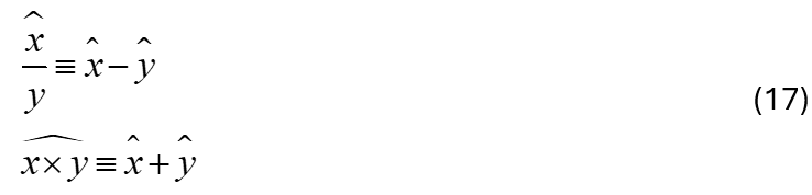
Macroeconomics abounds in ratios and products. These can be easily transformed into dynamic statements by log differentiation:

The notation can be simplified by defining:

Then:
A series of models can be constructed using this method, ranging from a simplest-possible model with only two system states (the employment rate and the share of wages in GDP) and linear behavioural equations, to a five-system state model (including private debt, the government deficit, and the price level) with nonlinear behavioural equations.
These models show that a pure private sector model, with no government sector, is susceptible to collapsing into a debt-deflation. In contrast, a system in which government spending can exceed taxation is immune to such crises:
we prove in Proposition 4 that under a variety of alternative mild conditions on government subsidies, the model describing the economy is uniformly weakly persistent with respect to the employment rate…
we can guarantee that the employment rate does not remain indefinitely trapped at arbitrarily small values. This is in sharp contrast with what happens in the model without government intervention, where the employment rate is guaranteed to converge to zero and remain there forever if the initial conditions are in the basin of attraction of the bad equilibrium corresponding to infinite [private] debt levels {Costa Lima, 2014 #5111`, p. 31}
The first set of models in this chapter abstract from price dynamics.
The Simplest Possible Model
Consider the simplest possible model of a capitalist system in which there are just two income sources—wages and profits. The two key definitions are the wages share of GDP (which is one minus the profit share), and the employment rate (which incorporates the effects of population and productivity growth). Defining the wages share as w and the employment rate as l, and using Y for GDP, W for total wages, L for employment and N for population, we have:

Applying log differentiation, we can convert these ratios into true-by-definition dynamic statements:
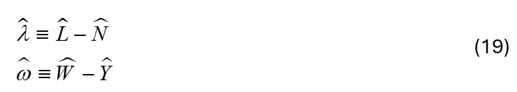
In words, these equations state that:
“The employment rate will grow if employment grows faster than population”; and
“The wages share of GDP will grow if wages grow faster than GDP”
These are still definitions, though expressed in dynamic form. In order to convert them into a model, we need some realistic simplifying assumptions to link the system states together. In this simplest possible model, these are that:
There is a uniform real wage rate w;
The rate of change of the wage rate is a linear function of the employment rate:

Output is a linear function of capital (K)—see Chapter 9 on page 67 for an empirical justification of this assumption:[1]

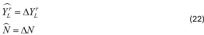
The output to labour ratio YLr and population grow exponentially:

All profits are invested, so that the rate of change of Capital equals profits minus depreciation, where depreciation is a linear function of capital :
Given the linear relationship between output and capital, the rate of growth Y is the same as the rate of growth of capital:


Derivation of the dynamics of the employment rate is straightforward:[2]

Here the bracketed term is the rate of real economic growth:
The derivation of the wages share of GDP is even simpler:
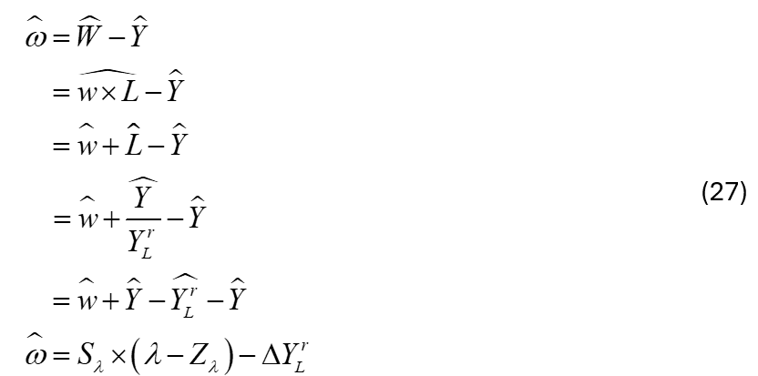
The resulting system is:

Figure 22 shows the dynamics of this model.

Figure 22: Basic 2D macro model generates sustained cycles
Stability analysis shows that the non-zero equilibrium of this system is neutral, since the system has complex conjugate eigenvalues with zero real part. This puts it in the class of predator-prey models first developed by Lotka {Lotka, 1920 #5973}, with—given the fact that this model was first developed by Richard Goodwin {Goodwin, 1967 #279;Goodwin, 1966 #5954} to put into mathematical form a verbal cyclical model developed by Marx {Marx, 1867 #1083`, Chapter 25}—the ironic twist that the capitalists are the prey, and the workers are the predators.
Including private debt
As the previous chapters have shown, private debt plays a critical role in macroeconomics. This is captured by replacing the simplifying assumption used above—that capitalists invest all their profits—with the more realistic assumption that capitalists invest more than profits during a boom, and less than profits during a slump. They borrow the difference from banks, and have to pay interest on the outstanding debt. In this model, profit is net of interest payments as well as of wages, and gross investment is now a linear function of the profit rate:

This makes the private debt ratio dr a third system state, which introduces the possibility of chaotic outcomes {Li, 1975 #1838}. Expressed as a dynamic equation, this definition states that the private debt ratio will rise if debt grows faster than GDP:

The rate of economic growth is given by Equation , leaving just the rate of growth of the debt ratio to be derived. In this model is it is set equal to gross investment minus profits—an assumption which is supported by empirical research by Fama and French {Fama, 1999 #3976}:
The source of financing most correlated with investment is long-term debt. The correlation between and and is 0.79. The correlation between and net new short-term debt is lower, 0.60, but nontrivial. These correlations confirm the impression … that debt plays a key role in accommodating year by-year variation in investment. {Fama, 1999 #1845`, p. 1954}
This suggests the following equation for the rate of change of private debt:

The derivation of this third system state is straightforward:

We therefore get:

The full system is:
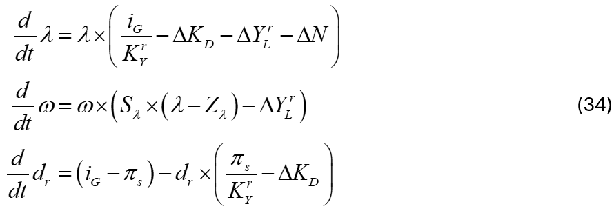
This system has two meaningful equilibria (the 3rd yields negative values for the private debt ratio), one of which has positive values for the employment rate, wages share and private debt ratio, and the other has zero employment rate and wages share and an infinite debt ratio—because GDP converges to zero while private debt remains positive.
The former equilibrium was dubbed the “Good Equilibrium” and the latter the “Bad Equilibrium” by the mathematicians Matheus Grasselli and Bernard Costa-Lima—see their paper {Grasselli, 2012 #4059} for a full exposition of the dynamics.
The Good Equilibrium is a strange attractor: it has one negative real eigenvalue, and two complex conjugate eigenvalues which, for realistic parameter values, have a positive real part. From a distance the real eigenvalue dominates, but on approach the positive real part of the complex eigenvalues dominates. The system therefore cyclically approaches the Good Equilibrium, only to be cyclically repelled from it on approach, after which the system has rising cycles for a while until it falls into the basin of attraction of the Bad Equilibrium—see Figure 23.
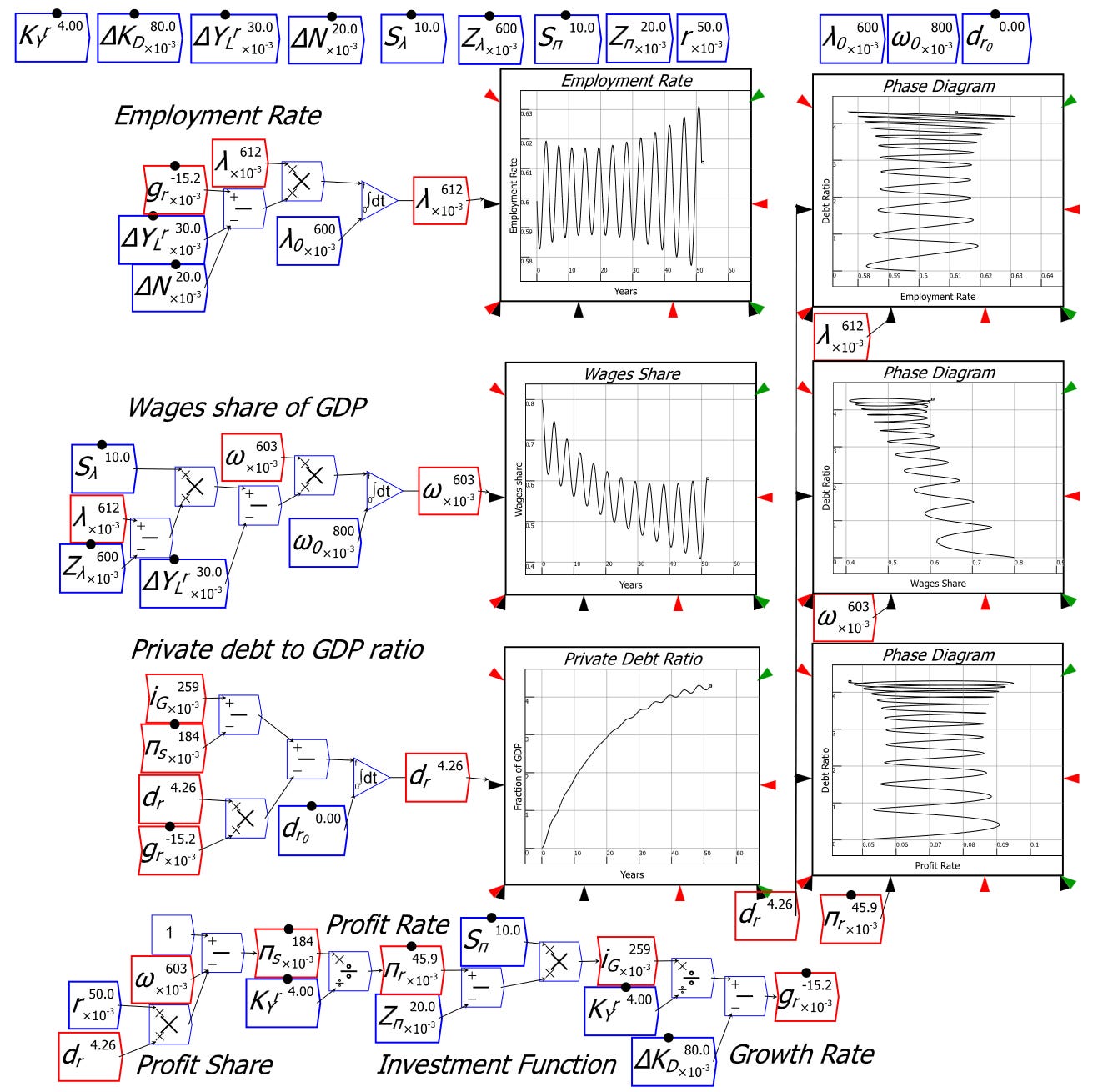
Figure 23: 3D model with private debt can undergo a debt-induced collapse
This system has two emergent properties, both of which occurred in the empirical data of the Global Financial Crisis: the crisis is preceded by a period of falling volatility, and the increase in private debt occurs at the expense of the workers’ share of GDP, even though workers do not borrow in this model.
Including government deficit spending
We now add a government sector whose spending in excess of taxation revenue is driven by the rate of employment—as shown empirically in the previous chapter.
The first issue is how to account for government deficit spending in the distribution of income. This was solved by the Polish engineer-turned-economist Michal Kalecki by a series of comparisons of the income and expenditure measure of GDP {Kalecki, 1954 #7115`, pp. 45-49}.
Kalecki started with dividing society into capitalists and workers. This gave 2 sources of income—wages and profits—and three categories of expenditure—workers consumption, capitalists consumption, and investment: see
Table 5: Kalecki's initial derivation of the aggregate sources of profits

Kalecki commenced his analysis with the simplifying assumption that workers spend all their incomes led to the equation:

He then reasoned that causation ran from right to left—that capitalists consumption plus investment determined profits:
it is clear that capitalists may decide to consume and to invest more in a given period than in the preceding one, but they cannot decide to earn more. It is, therefore, their investment and consumption decisions which determine profits, and not vice versa. {Kalecki, 1954 #7115`, p. 46}
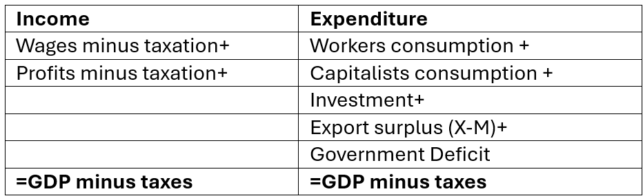
Next he included government spending and taxation, and exports minus imports:
Table 6: Stage two: including government and the foreign sector

Deducting Taxes from both columns enabled him to introduce the government deficit:
Table 7: Stage two: including government and the foreign sector
Relaxing the assumption that workers spend all their incomes led to what is known as the Kalecki Profit Equation:

For our purposes, this indicates that the government deficit adds to profits, so that the profit share equations are now:

And

Where

We now need a function for government spending as a function of the employment rate, where spending falls as the rate of employment rises. A linear equation (nonlinear functions will be introduced shortly) is:
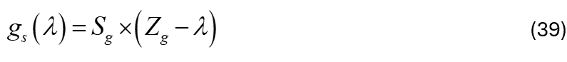
The government spending ratio equation can be given a verbal interpretation akin to those for the employment rate, wages share of GDP, and private debt ratio:
“The government deficit to GDP ratio will rise if the deficit rises faster than GDP”
Solving for

Therefore

The system with government and linear behavioural function is:

This system is simulated in Figure 24, with government spending turned on at the 75 year mark. Government deficit spending prevents the system collapsing into a private debt crisis which occurred with the private-sector-only model in Figure 23. This was confirmed as an inherent property of the model by the mathematicians Costa Lima and Grasselli, using persistence theory, in “Destabilizing a stable crisis: Employment persistence and government intervention in macroeconomics”:
we can guarantee that the employment rate does not remain indefinitely trapped at arbitrarily small values. This is in sharp contrast with what happens in the model without government intervention, where the employment rate is guaranteed to converge to zero and remain there forever if the initial conditions are in the basin of attraction of the bad equilibrium corresponding to infinite [ratio to GDP, private] debt levels. {Costa Lima, 2014 #5111`, p. 31}

Figure 24: 4D model including government deficit spending with linear behavioural functions
Some unrealistic aspects of this model—notably, the government deficit hitting 30% of GDP—are the product of the linear behavioural functions used in the model. Replacing these functions with suitable nonlinear functions, such as the generalised exponential functions shown in Figure 25, results in both more realistic values, and more complex systemic behaviour.

Figure 25: Nonlinear Behavioural functions for wages, investment and the government deficit
Rather than convergence to equilibrium, as in the linear case, nonlinear behavioural functions lead to sustained cycles—see Figure 26. This illustrates that stability in a complex system is better seen as the absence of breakdown—in mathematical terms, the persistence of all system states in the model—rather than the absence of cycles.

Figure 26: Sustained cycles but no breakdown in the government model with nonlinear behavioural functions
This definitional approach to macroeconomics reaches several conclusions which are antithetical to the conventional treatment of macroeconomics, both in the form of IS-LM-based models before the “microfoundations revolution” in economics, and DSGE models since:
The economy is inherently cyclical, versus the equilibrium orientation of conventional economics;
The primary danger to the survival of a capitalist economy is a private debt crisis, not a government debt crisis; and
Countercyclical government spending can make that outcome impossible, whereas it is possible in either a pure private enterprise economy, or one in which the government spending is not countercyclical.
This hints at an evolutionary explanation for the dramatic increase in the scale of government spending and taxation over the last century. In the 19th and early 20th centuries, government spending was a trivial fraction of GDP—as shown by Figure 27—and deflationary crises were a regular occurrence. As Hyman Minsky put it:
Before World War II, serious depressions occurred regularly. The Great Depression of the 1930s was just a "bigger and better" example of the hard times that occurred so frequently. This postwar success indicates that something is right about the institutional structure and the policy interventions that were largely created by the reforms of the 1930s. {Minsky, 1982 #35`, p. xi}
Part of that “institutional structure” was a far higher level of government spending and taxation. Both rose sharply across WWI, the Great Depression, and WWII, from 2% of GDP to of the order of 20% of GDP—see Figure 27.

Figure 27: The government spending to GDP ratio increased tenfold after 1917
Though it is easy to interpret this as due solely to bureaucratic overreach, it is arguable that it was a systemic response to those crises, in which deflation played a major role. Contrary to popular folklore that the Weimar inflation led to Hitler’s rise to power, his ascension was preceded by a period of deflation as severe as the US experienced during the Great Depression—see Figure 28.

Figure 28: Hitler's rise to power was preceded by deflation, not inflation
This raises the issue of what happens to the dynamics detailed in this chapter when prices are included in the models. This is the topic of the next chapter.
[1] This is an empirically derived relation first noted by Leontief {Leontief, 1937 #7014}, which can be shown to be based upon the role of machinery in enabling energy to be turned into useful work. Neoclassical economists habitually use the Cobb-Douglas Production Function, but this function is invalid for reasons that I detail in Chapter 13 of Rebuilding Economics from the Top Down (which is available at https://tinyurl.com/y8uvt676).
[2] And far simpler than what Blanchard accurately described as the “long slog from the competitive model to a reasonably plausible description of the economy” which Neoclassical economists face when they attempt to derive macroeconomics algebraically from microeconomics.