Equilibrium (is) for Dummies

In recent months, there has been a resurgence of Neoclassical economists tweeting about equilibrium, and championing their approach to economics over that of heterodox economists like me. This includes both established academics, and new graduates from undergraduate degrees.

Here’s the “Howard Marks Presidential Professor of Economics at the University of Pennsylvania”, Jesus Fernandez-Villaverde, asserting that anyone who doesn’t know what an equilibrium is—as defined by Neoclassical economics—should be ignored:

University of Warwick Professor of Economics Roger Farmer chimed in as well, asserting that “An economic model requires an EQUILIBRIUM CONCEPT”:

At the other end of the economics pecking order, a recent graduate economist opined that “Economics is possible as a scientific study only if the economy has a prevailing tendency to move toward equilibrium”

Equilibrium, equilibrium, equilibrium…

I wondered why this was happening now, and then I realized that we are approaching the 20^th anniversary of the Global Financial Crisis. It will soon be 20 years since the most recent spectacular failure of Neoclassical economics—the failure to anticipate the biggest economic crisis since the Great Depression.

Far from indicating where the economy was actually headed—into a severe economic downturn—their models told them that a great year lay ahead. This was Bernanke’s Report to Congress on July 18, 2007—just 3 weeks before the crisis began on August 9, 2027:

The U.S. economy seems likely to continue to expand at a moderate pace in the second half of 2007 and in 2008… forecasts for the increase in real GDP [are] 2¼ percent to 2½ percent over the four quarters of 2007 and 2½ percent to 2¾ percent in 2008. (Bernanke 2007)

This spectacularly wrong prediction—the rate of economic growth in 2008 was not 2.75 percent but minus 2.5 percent, and the recession he didn’t see coming was the longest in US post-WWII history—was not unique to Bernanke. Virtually all Neoclassical economists were caught completely by surprise by the crisis (Robert Shiller was about the only exception), and for the next decade many posts by Neoclassical economics wondered whether their “Dynamic Stochastic General Equilibrium” models were fit for purpose.

But 20 years later, they’re back selling equilibrium analysis as if the GFC didn’t happen. Their students are falling for it, because they were infants when the GFC hit. They don’t have the experience or the memory to realise that this approach has been tested and failed, and they fall for the apparent but illusory sophistication of the mathematics.

Their predecessors did the same thing after The Great Depression: 20 years after it happened, they revived the equilibrium approach to economics that had failed them in the 1920s. This is despite the most famous Neoclassical economist of the time, Irving Fisher, concluding that equilibrium thinking was the problem:

Theoretically there may be—in fact, at most times there must be—over- or under-production, over- or under-consumption, over- or under spending, over- or under-saving, over- or under-investment, and over or under everything else. It is as absurd to assume that, for any long period of time, the variables in the economic organization, or any part of them, will stay put, in perfect equilibrium, as to assume that the Atlantic Ocean can ever be without a wave. (Fisher 1933)

Fisher’s criticisms of equilibrium economic analysis in the 1930s were ignored, and ironically, the definition of equilibrium that Fernandez-Villaverde asserts you have to know, and understand, and use today to be worth taking seriously on economics, is Fisher’s definition, which Fisher rejected because it led him into catastrophe in the Great Crash of 1929!

Similarly, Farmer champions John Hicks’s definition of economic dynamics as a sequence of equilibria over time:

I organize all of my thinking around the concept of *temporary equilibrium theory*, an idea that dates to Hicks’ book ‘Value and Capital’ (and perhaps earlier).

Clearly, Farmer is not aware that Hicks also rejected the use of equilibrium models in economics. Writing in the early 1980s, Hicks said, in reference to the first major post-World War economic crisis, that:

We know that in 1975 the system was not in equilibrium. There were plans which failed to be carried through as intended; there were surprises. We have to suppose that … It is sufficient to treat the economy … as if it were in equilibrium… we are accustomed to permitting ourselves this way out. But it is dangerous. Though there may well have been some periods of history, some “years,” for which it is quite acceptable, it is just at the turning points, at the most interesting “years,” where it is hardest to accept it. (Hicks 1981)

These economists, who think they’re doing advanced modelling, are in fact stuck in an intellectual cul-de-sac which is primitive from the point of view of modern mathematics. About sixty years ago, scientists and mathematicians discovered “complex systems”: extremely simple models could generate behaviour which could not be generated using equilibrium methods. The first was Lorenz’s model of fluid dynamics (Lorenz 1963). It was a deliberately simple model with just three variables and three parameters. Avert your eyes if equations aren’t your thing, but this is just about the simplest system you can imagine. There are just 3 variables (x, y, and z) and three constants (a, b and c), so it’s hard to imagine that this model could generate anything interesting:

In fact, it generates incredibly complex dynamics, which gave rise to the cliché of “the butterfly effect”. There are 3 equilibria in this model—the two “eyes” in the butterfly wings, and (0,0,0)—and they are all unstable. Therefore, the system remains “far from equilibrium” indefinitely.

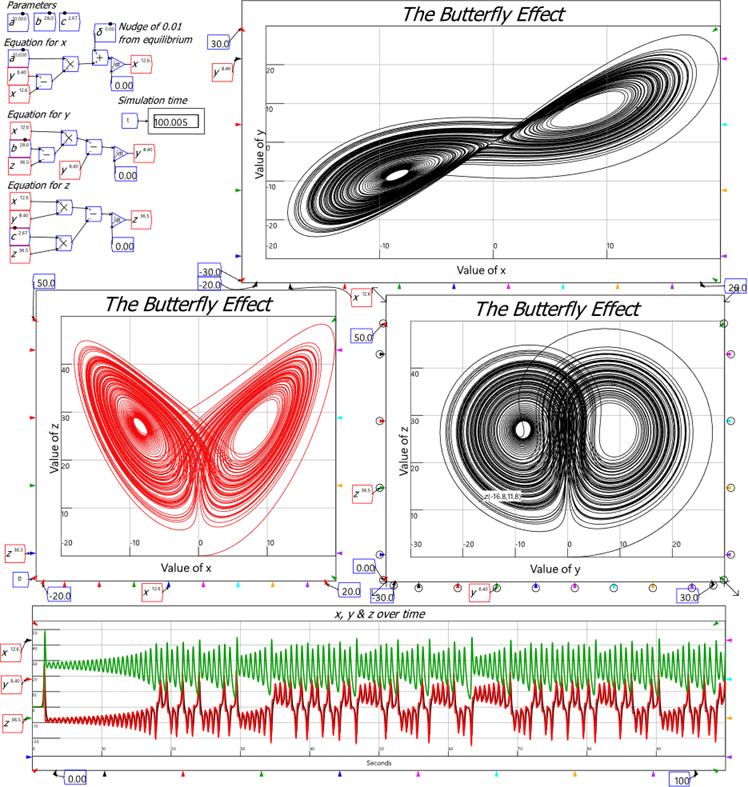
Figure 1: The strange attractor behaviour in Lorenz’s model of fluid dynamics

Their behaviour makes a mockery of how Neoclassical economists think about equilibrium, by showing the existence of what are now called “Strange Attractors”: equilibria that attract from a distance, but repel from close up.

This model clearly does not have “a prevailing tendency to move toward equilibrium”, to quote the recent graduate’s assertion, and yet this model is part of the foundation of modern meteorology—which is a far more trustworthy discipline than economics. This is because meteorologists embraced this discovery when it was made. Meteorologists abandoned the equilibrium and pattern-matching approaches they used to use. They accepted that the weather was an unstable system and then refined their capacity to model it.

To rework the recent graduate’s statement in the light of modern mathematical knowledge:

Equilibrium analysis is only possible as a scientific method if the economy has a prevailing tendence to move towards equilibrium. Since it doesn’t, nonequilibrium analysis is the correct scientific method for economics.

Why have economists resisted this? Largely because they have turned equilibrium from a convenient modelling technique in the days before computers, into a quasi-religious belief about the nature of a capitalist economy.

This is not how Neoclassical economics began. Its founders in the 19^th century all treated equilibrium as a wildly inaccurate characterisation of a capitalist economy, but what else could they do with just pen and paper? Jevons, who developed the marginal approach that characterizes Neoclassical economics, was emphatic that out-of-equilibrium dynamics was the correct method for economics, and that equilibrium analysis was a stop-gap:

We must carefully distinguish, at the same time, between the Statics and Dynamics of this subject. The real condition of industry is one of perpetual motion and change. Commodities are being continually manufactured and exchanged and consumed. If we wished to have a complete solution of the problem in all its natural complexity, we should have to treat it as a problem of motion—a problem of dynamics. But it would surely be absurd to attempt the more difficult question when the more easy one is yet so imperfectly within our power. (Jevons 1888)

JB Clark, who developed the marginal productivity theory of income distribution, described thinking in equilibrium terms about capitalism as “Heroically theoretical”—and not in the positive sense of a Homerian hero:

A static state is imaginary. All actual societies are dynamic; and those that we have principally to study are highly so. Heroically theoretical is the study that creates, in imagination, a static society. Unceasing changes in the actual world thrust labor and capital, from time to time, out of one occupation and into another. (Clark 1898)

There is no excuse today for using equilibrium methods to models the economy. Nonequilibrium tools exist and are widely used in real sciences. Nor is there any justification for trying to derive macroeconomics from microeconomics. This is another belief of Neoclassicals that scientists long ago realised was a fools errand. The real Nobel Prize winner Philip Anderson put this brilliantly over 50 years ago:

The main fallacy in this kind of thinking is that the reductionist hypothesis does not by any means imply a “constructionist” one: The ability to reduce everything to simple fundamental laws does not imply the ability to start from those laws and reconstruct the universe… Psychology is not applied biology, nor is biology applied chemistry (Anderson 1972)

And yet economists believe that macroeconomics is applied microeconomics. Partially this is because they can’t think of any other way to build macroeconomic models. According to Olivier Blanchard, ex-Chief Economist of the IMF:

The pursuit of a widely accepted analytical macroeconomic core, in which to locate discussions and extensions, may be a pipe dream, but it is a dream surely worth pursuing. If so, the three main modeling choices of DSGEs are the right ones. Starting from explicit microfoundations is clearly essential; where else to start from? (Blanchard 2016)

In fact, macroeconomics can be derived directly from macroeconomic definitions—and what emerges is not Neoclassical economics, but the core models from my side of economics, the so-called “Post-Keynesian” school. The key definitions are the employment rate, the wages share of GDP, the private debt ratio, and the ratio of government deficit spending to GDP. I explain why these are the key factors in my online course, but briefly:

• The employment rate is a key factor in all economic models, and it is dependent on the level of output and the state of technology;

• The wages share of GDP brings in the distribution of income;

• The private debt level relative to GDP measures the impact of finance sector on the economy; and

• The government deficit relative to GDP measures the impact of the government on the economy.

Extremely simple mathematics—which I’ll detail at the end of this post—converts these definitions into obviously true dynamic statements:

• The employment rate will rise if employment grows faster than population;

• The wages share of GDP will rise if wages grow faster than GDP;

• The private debt ratio will rise if debt grows faster than GDP; and

• The government deficit to GDP ratio will rise if the government deficit grows faster than GDP.

These are all still true-by-definition statements; they’ve just been converted to dynamic statements. To make models out of these definitions, you need to add some realistic simplifying assumptions:

• Workers capacity to get wage rises are a positive function of the rate of employment;

• Firms desire to invest is a positive function of the rate of profit; and

• The government deficit ratio is a negative function of the rate of employment

Three canonical Post-Keynesian models result.

With just employment and wages share, we get Goodwin’s “growth cycle” model of employment versus the wages share of GDP. This shows capitalism as an inherently cyclical system. The core equilibrium of this model is neutral—it neither attracts nor repels the system.

Figure 2: Goodwin’s cyclical model of the economy, derived from macroeconomic definitions

With the private debt ratio, we get Minsky’s Financial Instability Hypothesis: capitalism can collapse into a debt-deflation as a series of booms and busts leads to a private debt ratio that overwhelms the economy.

Figure 3: Minsky’s “Financial Instability Hypothesis”, derived from macroeconomic definitions

With the government deficit included, we get a complex-systems version of “Modern Monetary Theory”: government counter-cyclical spending can prevent a debt-deflation, but it results in complex cycles rather than an equilibrium.

Figure 4: A complex systems version of MMT, derived from macroeconomic definitions

This is the correct way to build macroeconomics, and Neoclassicals, with their equilibrium fetish, their false belief that macroeconomics must be derived from microeconomics, and their empirically false microeconomics, are holding us back from it.

If you’ve survived this far into this post, I’ll now explain how this approach to macroeconomics works, using the first model as an example.

Macroeconomics from Macroeconomic Definitions

The definition of the Wages Share of GDP is:

This also means that the percentage rate of change of the wages share of GDP is equal to the percentage rate of change of that ratio. Using a “hat” (Ù) symbol to indicate the percentage rate of change of a variable, we get

One rule of percentages can now be applied: the percentage rate of change of a ratio is the percentage rate of change of the numerator minus the percentage rate of change of the denominator:

Now we bring in our first assumption: a uniform wage rate (in later models, this can be made more realistic by using a vector of wage rates, in a multi-commodity model of the economy). Therefore:

The same percentage rate of change rule applies:

Another rule of percentages applied to products is that the rate of change of a product equals the sum of the rates of change of its components:

Feed this back into the Wages Share equation and we have

Since employment depends on GDP, we can define a GDP to Employment ratio:

Therefore we can define Employment as:

Substitute this back into the Wage Share equation and we get:

Expand this term using the rule of percentages and we get:

The GDP terms cancel, and we’re left with:

That is the first of the two dynamic equations in this simple definitions-based model. To complete it, I need causal relationships for both the rate of change of the wage rate and the rate of change of the GDP to employment ratio.

The rate of change of the wage rate depends on the employment rate:

The simplest way to model this is as a linear relationship between the employment rate and the rate of change of wages. As Phillips insisted, the relationship is certainly nonlinear, and has at least 3 determinants rather than just one (Phillips 1958), but a linear relationship is sufficient to show the basic dynamics.

If you’ve gotten this far, I’m going to assume that you can cope with some symbols rather than full words (but I’ll revert to words for the derivation of the employment rate equation). I try to make symbols in my equations interpretable, so I use a range of symbols and formatting that is easy to interpret. I use the Greek capital D, D, to represent change. Lowercase w stands for the wage, the Greek lowercase l, l, stands for the employment rate. I use S for the slope of a line, Z for the zero intercept for a line, and subscripts to show which line I’m talking about. Since this is an equation for the rate of change of wages as a function of the employment rate, I use S_l and Z_l:

The rate of change of the GDP to Employment ratio is a measure of technical progress over time. As a first approximation, I assume that this is a constant. For a symbolic rendition of the GDP to Employment ratio, I use Y for GDP, subscripted L for Employment, and a superscripted lowercase r to show that this is a ratio:

Using the Greek lowercase w, w, for the wages share of GDP, this gives the final form of the first equation:

The second equation starts from the definition of the employment rate:

Applying the same percentage rules, we get:

Introducing the GDP to Employment ratio again and using the percentage rule again gives us:

Now GDP growth doesn’t cancel out, and we have to make assumptions about what causes the economy to grow. Here, I use the empirical regularity first observed by Leontief, when he developed input-output analysis in the 1930s and 1940s, that the ratio of GDP to the capital stock was roughly constant for each country he considered. That same relationship holds today, with a slight downward secular trend—see Figure 5.

Leontief didn’t have an explanation for this regularity, and Neoclassical frequently rubbish it, claiming that their preferred model of production—the Cobb-Douglas Production Function (CDPF)—is superior. I won’t cover these topics here—because this post is long enough already. But in recent years, I’ve shown, firstly that Leontief’s ratio is based on the efficiency with which machinery turns energy into useful work (Keen, Ayres, and Standish 2019), and secondly, that the derivation of the CDPF was based on egregious statistical errors (Keen 2025, pp. 74-83). If Cobb had done his analysis correctly, the original Cobb-Douglas paper (Cobb and Douglas 1928) would never have been submitted to a journal, let alone become as influential as it is today.

Figure 5: US Capital to Output ratio as estimated by Penn World Tables

I now introduce the ratio, between GDP and Capital, where this ratio is assumed to be a constant:

Therefore, the rate of growth of GDP equals the rate of change of capital:

The employment rate equation is now:

Using K for the number of machines, the percentage (or fractional) rate of change of capital is:

The rate of change of capital is net investment, which equals gross investment minus depreciation:

Measured depreciation of physical capital is a fraction of existing capital, and the rate of depreciation is normally measured at about 6% p.a. That leaves gross investment to consider, and the simplifying assumption that Goodwin made was the best possible one for a capitalist system: he assumed that capitalists invest all their profits. Since profits in this simple model are equal to output minus wages, we can write:

Using Y for GDP, W for total wages, and DK_D for the rate of deprecation, the expression for the rate of change of the Capital stock can be written:

Feeding this back into the equation for the rate of change of the employment rate, we have:

Using K_Y^r for the Capital to GDP ratio, we get:

(Y-W)/Y is one minus the wages share of GDP. This lets us arrive at the final form of the model:

That’s the model simulated in Figure 2, which Goodwin derived in a much more complicated way. With the method of working from definitions, it takes minutes to build this model—and that’s with no need to learn the ridiculous nonsense of Neoclassical microeconomics first. But there’s another way to reach the same result that doesn’t even require any algebra: it’s to build a system dynamics model of the economy using Ravel. Figure 6 shows the same model as in Figure 3, built using flowchart logic rather than algebraic manipulations of rate of change equations.

Figure 6: The 3D model with private debt as a flowchart in Ravel

The definitional approach, and system dynamics, work because they describe the structure of the economy—and that is what explains the cyclicality of the economy that we see in the real world, and that Neoclassicals misinterpret as due to “exogenous shocks”.

The equilibrium fetish of mainstream economics inhibits the development of realistic models like these, and keeps economists in the dark about the actual economy as they build their esoteric DSGE models, which assume that people can accurately anticipate an infinite-future.

I’ll finish on this note: poor victims of a conventional Neoclassical curriculum believe what they’re doing is science:

That’s because their textbooks, and the Neoclassical true believers that teach them, don’t tell them the batshit crazy assumptions that are made to try to escape the inescapable logical fallacies of Neoclassical economics. There are many such crazy assumptions, which I’ll cover in my next post. Of all of them, this is probably my favourite. It is how Debreu tried to evade the impact of time on his general equilibrium model:

For a producer … a production plan (made now for the whole future) is a specification of the quantities of all his inputs and all his outputs;… The certainty assumption implies that he knows now what input-output combinations will be possible in the future (although he may not know now the details of the technical processes which will make them possible)… (Debreu 1959, p. 38)

Neoclassicals gave him the “Nobel” Prize for this work. A padded cell would have been a more appropriate award.

References

Anderson, P. W. 1972. ‘More Is Different: Broken symmetry and the nature of the hierarchical structure of science’, Science, 177: 393–96.

Bernanke, Ben. 2007. “Monetary Policy Report to the Congress.” In. Washington: Federal Reserve.

Blanchard, Olivier. 2016. ‘Do DSGE Models Have a Future? ‘, Peterson Institute for International Economics. https://www.piie.com/publications/policy-briefs/do-dsge-models-have-future.

Clark, John Bates. 1898. ‘The Future of Economic Theory’, The Quarterly Journal of Economics, 13: 1–14.

Cobb, Charles W., and Paul H. Douglas. 1928. ‘A Theory of Production’, The American Economic Review, 18: 139–65.

Debreu, Gerard. 1959. Theory of value :an axiomatic analysis of economic equilibrium (Yale University Press: New Haven :).

Fisher, Irving. 1933. ‘The Debt-Deflation Theory of Great Depressions’, Econometrica, 1: 337–57.

Hicks, John. 1981. ‘IS-LM: An Explanation’, Journal of Post Keynesian Economics, 3: 139–54.

Jevons, William Stanley. 1888. The Theory of Political Economy ( Library of Economics and Liberty: Internet).

Keen, S. 2025. Money and Macroeconomics from First Principles for Elon Musk and Other Engineers (Ravelation: Netherlands).

Keen, Steve, Robert U. Ayres, and Russell Standish. 2019. ‘A Note on the Role of Energy in Production’, Ecological Economics, 157: 40–46.

Lorenz, Edward N. 1963. ‘Deterministic Nonperiodic Flow’, Journal of the Atmospheric Sciences, 20: 130–41.

Phillips, A. W. 1958. ‘The Relation between Unemployment and the Rate of Change of Money Wage Rates in the United Kingdom, 1861-1957’, Economica, 25: 283–99.